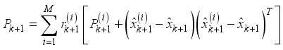
We have designed an interacting multi-model strong robust adaptive unscented Kalman filter for bearing only tracking of an underwater vehicle approaching the observer. To solve the problem of tracking an approaching underwater vehicle to the observer based on only its bearing, an interactive multi-model robust adaptive unscented Kalman filter is proposed in this paper. First, a new model of the bearing sense motion towards the observer is proposed to construct a set of realistic target motion modes consisting of linear and curved motion modes. In addition, to account for the influence of outliers in the target bearing measurements, the distribution of measurement noise is assumed to have a Student’s t-distribution, and the probability distribution of the degree of function and the scaling matrix of this distribution is assumed to have a gamma distribution and an inverse Wishart distribution. Thus, the model interaction step is to factorize the mixed probability density function using variational Bayesian method and, based on this, a predictive update method is proposed. In the measurement update phase, the posterior probability density function is obtained in factorization form using variational Bayesian method, and based on this, a posteriori mode probability calculation method is proposed. Simulation results show that our proposed method greatly improves the convergence rate of target tracking error.
| Published in | Engineering Mathematics (Volume 9, Issue 2) |
| DOI | 10.11648/j.engmath.20250902.13 |
| Page(s) | 46-67 |
| Creative Commons |
This is an Open Access article, distributed under the terms of the Creative Commons Attribution 4.0 International License (http://creativecommons.org/licenses/by/4.0/), which permits unrestricted use, distribution and reproduction in any medium or format, provided the original work is properly cited. |
| Copyright |
Copyright © The Author(s), 2025. Published by Science Publishing Group |
Bearing only Tracking, Unscented Kalman Filter, Inverse Wishart Distribution, Interactive Multi-Model
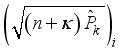
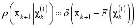
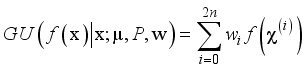
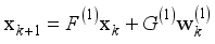
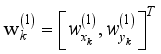
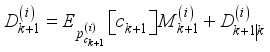
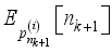
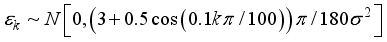
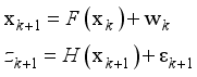 (1)
(1)  represents the
  moment (simply called
  moment),
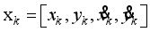
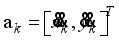
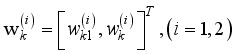
  is the state vector and the measurement of the system.
  is the sampling period,
  is the independent process noise vector and measurement noise.
  with mean
  and co-variance
  , UKF approximates
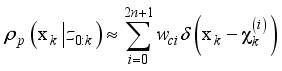
  by samples of the Gaussian density function
  respectively to perform a one-step prediction of the state quantity
  and co-variance
  , respectively, as follows
 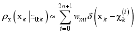 (2)
(2)  (3)
(3) 
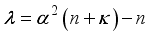 is the scale parameter,
  controls the deviation of sigma points and is usually set to a small parameter.
  is usually set to zero as a second-order scale parameter.
  is a dirac-delta function. For a Gaussian distribution,
  is optimal.
 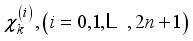 is obtained as follows.
 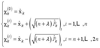 (4)
(4)  represents the
  -th column vector of the square root matrix of the matrix
  . Equation (4) is called the UT for computing the sigma points of
  from
from  .
.  is called a sigma point.
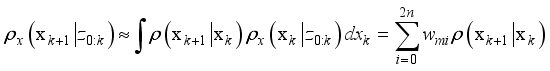
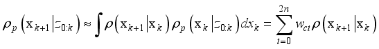
 , the predicted state becomes
 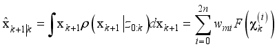 (5)
(5)  (6)
(6) 
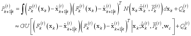
 (7)
(7)  is the sigma points distributed with co-variance
  centered around
  and
and  is the weight vector. This function is called the Gaussian integral approximation function using the UT and denoted by GU.
 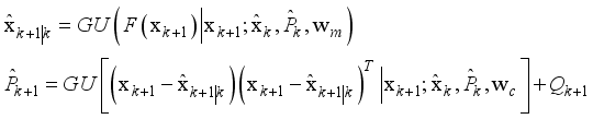 (8)
(8)  is a vector with
  as a component.
  to be a PDF on
  , the KL deviation of
  from
from  is defined as follows.
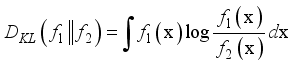 (9)
(9) 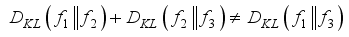 , in fact, KL deviation does not satisfy the range axiom.
  to call KL divergence.
  in the probability space
  is a PDF on
  with mean
  and co-variance
  ,
,  is a Gaussian PDF, we have
 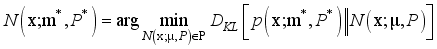 (10)
(10)  PDFs
PDFs  defined in the probability space
  , we define the weighted KL deviation as follows:
 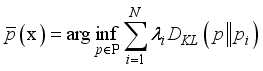 (11)
(11) 
 (12)
(12)  (13)
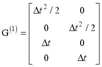
(13)  is the state transition matrix and
  is the noise gain matrix.
  ;
;  .
. 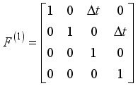 ,
,  (14)
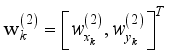
(14)  are mutually independent zero-mean white noises whose variances are all
  .
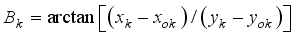
.  is the bearing, and
  ,
,  are the constant velocity of the underwater vehicle and the observer, respectively.
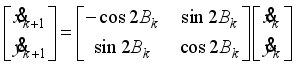
  .
.  can be written as follows:
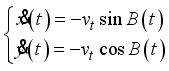
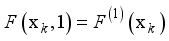
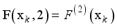
 , and if it is moving,
 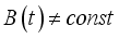 .
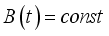
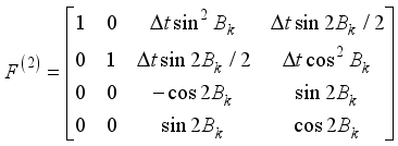
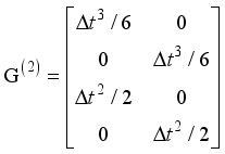
.  , the vehicle does not generally have a straight line motion, so that all components of acceleration are nonzero. Thus
 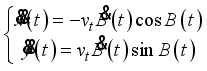 (15)
(15) 
 (16)
(16)  during
  .
.  obtained from Eq. (15) at time
  , the equation of motion of the underwater vehicle can be expressed as follows:
 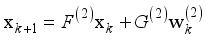 (17)
(17)  are mutually independent zero-mean white noises whose variances are all
 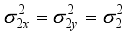 , and the state transition matrix
  is obtained by
 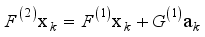 .
.  ,
,  (18)
(18)  (19)
(19)  in Eq. (16) varies with the position of the observer, as in Eq. (19), by means of the position vector
  of the observer, we can treat the position of the observer as the optimal state estimation problem of the underwater vehicle with the control signal.
 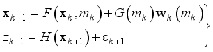 (20)
(20)  ,
,  ,
,  ,
,  ,
,  and
and  is the process noise co-variance.
  follows the Student’ t-distribution.
 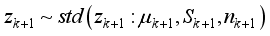 .
.  is the mean, scale matrix and the degree of function (DOF), respectively.
  can be written as follows
 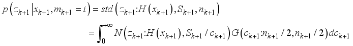 (21)
(21)  is the gamma PDF. Where
  is an auxiliary parameter.
  , we assume as follows:
  is gamma distributed.
  (22)
(22)  has a large value, the posterior distribution of DOF
  is assumed to be gamma distributed.
 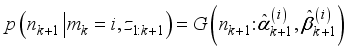 (23)
(23)  as follows.
  is the inverse Wishart distribution.
 is the inverse Wishart PDF,
  is the DOF, and
  is the inverse scaling matrix.
 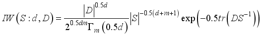 (24)
(24)  is the Di-gamma function and
  is the output number.
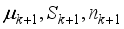
  , the state quantities
  , the scaling matrix
  , and the DOF
  are independent of each other.
  in Eq. (1) is independent of the state quantity at time
  , enabling the design of the new IMM filter we are going to propose.
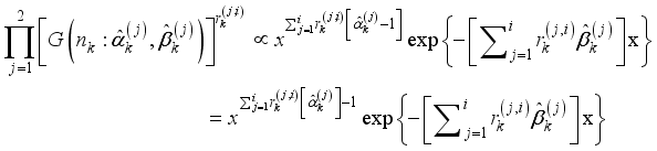
  , the predicted mode probability
  and the mixed probability
  have the following relations:
 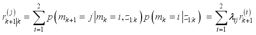 (25)
(25)  (26)
(26)  is the probability that the
  -th motion is converted to the
  -th motion
  and
and  becomes as follows:
 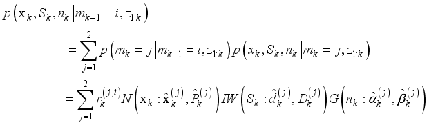 (27)
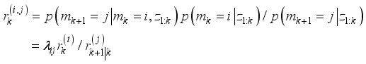
(27)  in the mixed PDF (27) is
 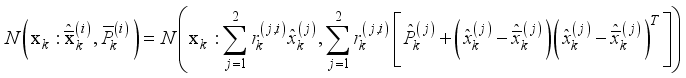 (28)
(28)  is
is 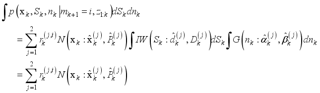 (29)
(29) 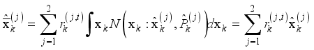 (30)
(30) 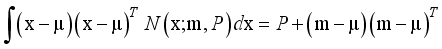 , the co-variance becomes
 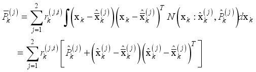 (31)
(31)  with the mean (30) and co-variance (31).
  and
and  in the mixed PDF (27) are obtained, respectively, as follows:
 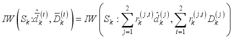 (32)
(32) 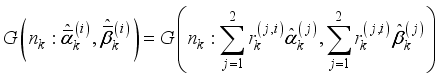 (33)
(33)  are respectively
 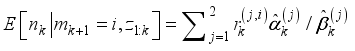 (34)
(34)  (35)
(35)  is
is 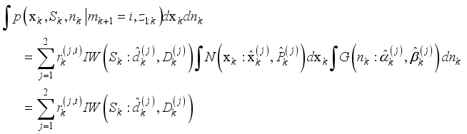 (36)
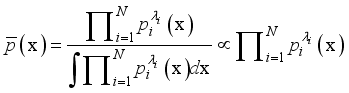
(36)  , the weighted KL deviation for two inverse Wishart PDFs
  with weight
  is given by Definition 2 and Lemma 2 as follows.
  (37)
(37)  is
is  (38)
(38)  (39)
(39)  are
are 
 respectively.
  (40)
(40)  (41)
(41)  by Eq. (39) has a gamma distribution, and hence from Eqs. (40) and (41) we obtain
 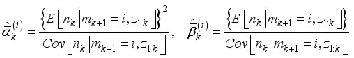 (42)
(42)  (43)
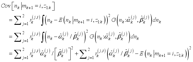
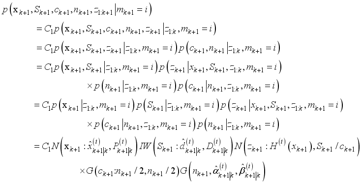
(43)  at time
  , and this predictive PDF is obtained by the champhman-Kolmogorov equation
  moment.
 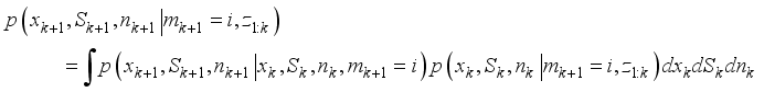 (44)
(44) 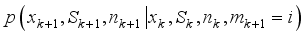 is a state transition PDF, and the distribution of the dynamic model, scale matrix and DOF that give the state transition can be considered independent of each other. Also, since the posterior PDF
 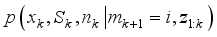 in (44) is a mixed PDF at the time
  shown in (43), we can write (44) as follows.
 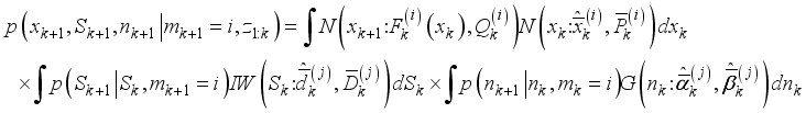 (45)
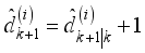
(45)  , the predicted state, the scaling matrix and the probability distribution of DOF are independent of each other and maintain the previous distribution patterns.
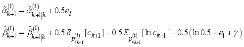
 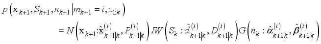 (46)
(46)  (47)
(47)  (48)
(48)  and
and  of the scaling matrix
  and the DOF
  are difficult to find directly by Eq. (45). This is because the dynamic model of the scale matrix and the DOF is usually unknown in practice, and the dynamics
  of the scale matrix and the DOF
  in Eq. (45) are not known exactly. Therefore, we propose heuristic dynamics for scaling matrices
  and DOF
  . This is the dynamics that simply spreads the previous approximation posterior of the scaling matrix
  and the DOF
 ,
,  that must be determined in the prediction step are determined by the following discovery dynamics such that in the measurement update step the posterior parameters
  ,
,  can be determined accurately by the fixed point iteration method. (see the IMM-SRAUKF algorithm)
 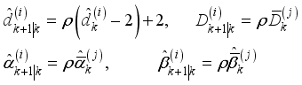 (49)
(49)  . We usually set
 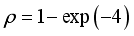 . The IMM-SRAUKF cannot estimate the process noise co-variance
  shown in Eq. (20) as the total mean of
  . One method is to dynamically adjust
  by fusing the past and the current of the co-variance matrix through the forgetting factor
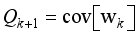
 (50)
(50)  .
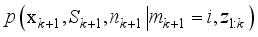
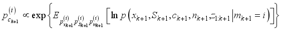
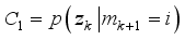
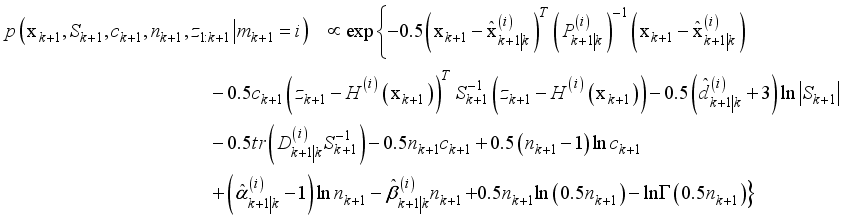
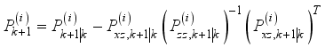
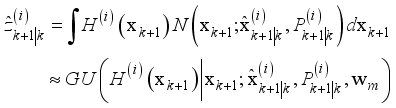
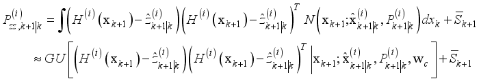
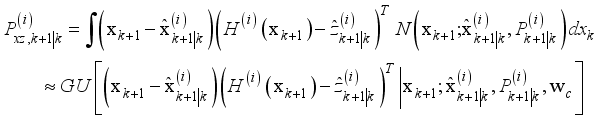
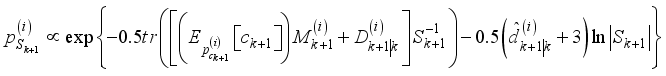
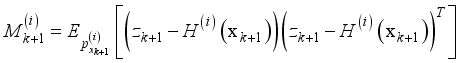
.  and the measurement are difficult to obtain analytically the posterior PDF, the measurement update step is to approximate the posterior PDF
  by using the VB approximation in the following factorized form, given the motion mode
  of the time
  and the new measurement
  .
.  (51)
(51)  (52)
(52)  are obtained by the VB approximation as the PDFs that minimize the KL deviation as follows:
 satisfying the above equation have the following forms:
  (53)
(53)  (54)
(54)  (55)
(55)  (56)
(56)  (57)
(57)  .
.  (58)
(58)  (59)
(59) 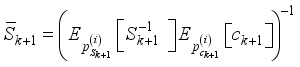 (60)
(60)  is the modified co-variance matrix. By Eq. (59), we can write the following relation:
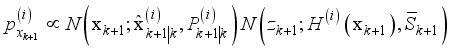
 can be written in the form of Gaussian PDF as
 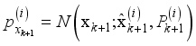 (61)
(61)  (62)
(62)  (63)
(63)  (64)
(64)  (65)
(65)  (66)
(66)  (67)
(67)  (68)
(68)  is an inverse Wishart PDF because
  has an inverse Wishart distribution. Thus, we have the following form of PDF:
 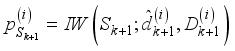 (69)
(69)  (70)
(70)  (71)
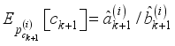
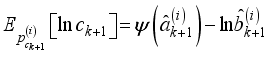
(71)  (72)
(72)  has a gamma distribution, so
  is a gamma PDF as follows:
 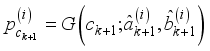 (73)
(73)  (74)
(74)  (75)
(75) 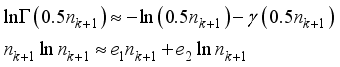 (76)
(76)  is the Euler gamma constant and
  is the least squares estimate. For example, for
  ,
,  ,
,  . Then Eq. (56) is obtained as follows:
  (77)
(77)  has the gamma PDF, so let us write this density function as
 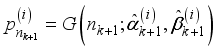 (78)
(78)  (79)
(79)  ,
,  ,
,  ,
,  ,
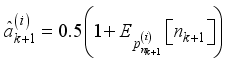
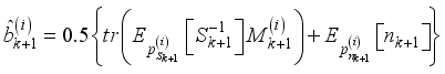
,  present in Eqs. (60), (68), (71), (74), and (75) are determined as follows:
 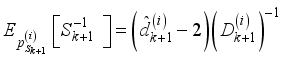 (80)
(80)  (81)
(81)  (82)
(82)  (83)
(83)  (84)
(84)  (85)
(85)  is a di-gamma function.
  and
and  in Eqs. (70) and (80), the problem of finding
  can be solved using the fixed point iteration method.
 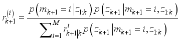 (86)
(86)  .
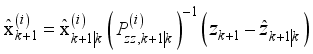
.  is determined by Eq. (25).
 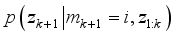 can be found as follows:
 (87)
(87)  (88)
(88) 
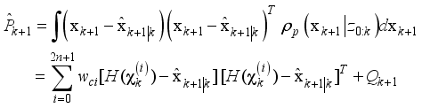
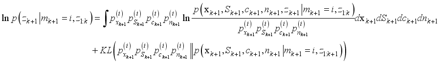
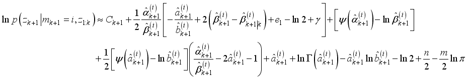
 shown in Eq. (88). Thus, the final state estimator and co-variance matrix are determined as follows:
 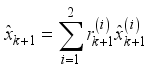 (89)
(89)  (90)
(90)  for each mode of motion
  and the forgetting factor
  of Eqs. (49) and (50). Let
  and go to step 2.
  and the mixed mode probability
  are calculated. Then, the mixing quantities
  are calculated using Eqs. (30)-(32), (42).
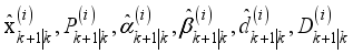
 in each mode using the fixed point iteration method shown in Figure 2.
 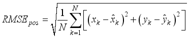 (91)
(91)  (92)
(92)  , the linear motion mode
  and the Bearing sense motion mode
  . The sampling period
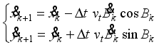
  . The simulation time interval is 0~200s. Figure 4 shows the motion trajectory of the observer and the target. The sight range of the day (SRD) was given as 6000 m.
  and radius SRD in the coordinate system shown in Figure 4, and the target is assumed to have a linear motion for 100 s and then a bearing sense motion towards the observer. To evaluate the performance of the proposed filter in tracking an underwater vehicle approaching the observer in two dimensions, we compare the tracking performance in three measurement noises.
  and the initial posterior mode probability by
  respectively. The initial state and covariance matrix are given as follows:
  ,
, 
 for process noise is the Gaussian noise with zero and co-variance
  . In the simulation, The Co-variance is assumed unknown. The forgetting factor of Eqs. (49) and (50) is given by
  , respectively, the initial parameter of the inverse Wishart distribution is given by
  , respectively, and all other initial parameters are given by 0.5.
  and the target velocity is constant
  .
. 
 . In Figure 5, the modal probabilities for the linear and bearing sense motions obtained by the proposed method are shown.


Case | IMM-CKF | IMM-UKF | IMM-VBF | Proposed method |
|---|---|---|---|---|
a | 16.3853 | 12.5860 | 15.7735 | 6.7743 |
b | 15.1209 | 10.9820 | 15.0893 | 5.0908 |
c | 19.4562 | 13.8467 | 17.3328 | 7.0835 |
Case | IMM-CKF | IMM-UKF | IMM-VBF | Proposed method |
|---|---|---|---|---|
a | 0.1092 | 0.1078 | 0.1001 | 0.0733 |
b | 0.1352 | 0.9677 | 0.0992 | 0.0912 |
c | 0.2921 | 0.8110 | 0.1191 | 0.1164 |
UKF | Unscented Kalman Filter |
CKF | Cubature Kalman Filter |
IMM | Interacting Multiple Models |
2D | Two-Dimensional |
Probability Density Function | |
VB | Variational Bayesian |
UT | Unscented Transform |
IMM-SRAUKF | Interacting Multi-Model Strong Robust Adaptive Unscented Kalman Filter |
KL | Kullback-Leibler |
DOF | Degree of Function |
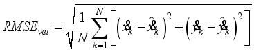
RMSE | Root Mean Square Errors |
SRD | Sight Range of the Day |
IMM-UKF | Interacting Multi-Model Unscented Kalman Filter |
IMM-CKF | Interacting Multi-Model Cubature Kalman Filter |
IMM-VBF | Variational Bayesian-based IMM Filter |
| [1] | X. Rong Li, Vesselin P. Jilkov, “Survey of Maneuvering Target Tracking. Part I: Dynamic Models,” IEEE Transactions on Aerospace and Electronic Systems, vol. 39, no. 4, pp. 1333- 1364, October 2003. IEEE Log No. T-AES/39/4/822061. |
| [2] | Dongliang Peng, Yunfei Guo, “Fuzzy-logic adaptive variable structure multiple-model algorithm for tracking a high maneuvering target,” Journal of the Franklin Institute, vol. 351, pp. 3837-3846, 2014. |
| [3] |
A. B. Miller, B. M. Miller, “Underwater Target Tracking Using Bearing-Only Measurements”, Journal of Communications Technology and Electronics, Vol. 63, No. 6, pp. 643–649, 2018.
https://doi.org/10.1134/S106422 6918060207 |
| [4] | Benlian Xu, Zhengyi Wu, Zhiquan Wang, “Theoretic Performance Bound for Bearings-Only Tracking”, Proceedings of the Sixth International Conference on Machine Learning and Cybernetics, Hong Kong, PP. 19-22, August 2007. |
| [5] | Kutluyıl Dogancay, “Bias Compensation for the Bearings-Only Pseudo linear Target Track Estimator”, IEEE Transactions on Signal Processing, vol. 54, no. 1, January 2006. |
| [6] | Zhao Li, Yidi Wang, Wei Zheng, “Adaptive Consensus-Based Unscented Information Filter for Tracking Target with Maneuver and Colored Noise”, Sensors, vol. 19, 2019. |
| [7] | Zhuoran Zhang, Changqiang Huang, Dali Ding, Shangqin Tang, Bo Han, Hanqiao Huang, “Hummingbirds optimization algorithm-based particle filter for maneuvering target tracking”, Nonlinear Dynamics, vol. 13, June 2019. |
| [8] | Jincheng Wang, Lei Xia, Lei Peng, Huiyun Li, Yunduan Cui, “Efficient Uncertainty Propagation in Model-Based Reinforcement Learning Unmanned Surface Vehicle Using Unscented Kalman Filte”, Drones, vol. 7, 2023. |
| [9] | J. Tague, “Detection of Target Maneuver from Bearings-Only Measurements”, IEEE Transactions on Aerospace and Electronic Systems”, vol. 49, no. 3, July 2013. IEEE Log No. T-AES/49/3/944629. |
| [10] | Dong Hui, Yang Wang Fang, Xiang Gao, “Target Tracking Method with Bearing-only measurements based on Reinforcement Learning”, IEICE Communication Express, vol. 5, no. 1, pp. 19-26, 2016. |
| [11] | Waqas Aftab, Lyudmila Mihaylova, “A Learning Gaussian Process Method for Maneuvering Target Tracking and Smoothing”, IEEE Transactions on Aerospace and Electronic Systems, vol. 57, no. 1, February 2021. |
| [12] | M. T. Sabet, A. R. Fathi, H. R. Mohammadi Daniali, “Optimal design of the Own Ship maneuver in the bearing-only target motion analysis problem using a heuristically super vised Extended Kalman Filter”, Ocean Engineering, vol. 123, pp. 146–153, 2016. |
| [13] | Wu Hao, Chen Shu Xin, Yang BFeng, Luo Xi, “Robust Range Parameterized Cubature Kalman Filter for Bearings-only Tracking”, J. Cent. South Univ., vol. 23, pp. 1399-1405, 2016. |
| [14] | Renke He, Shuxin Chen, Hao Wu, Zhuowei Liu, Jianhua Chen, “Robust maneuver strategy of observer for bearings‐only tracking”, Asian J. Control, pp. 1-13, 2013. |
| [15] | Thomas Northardt and Steven C. Nardone, “Track-Before-Detect Bearings-Only Localization Performance in Complex Passive Sonar Scenarios: A Case Study”, IEEE Journal of Oceanic Engineering, |
| [16] |
S. Koteswara Rao, “Bearings-only Passive Target Tracking: Range Uncertainty Ellipse Zone”, IETE Journal of Research,
https://doi.org/10.1080/03 772063.2020.1739571 |
| [17] | Singer, R. A, “Estimating optimal tracking filter performance for manned maneuvering target.” IEEE Transactions on Aerospace and Electronic Systems, Vol. 6, pp. 473-483, 1970. |
| [18] | H. A. P. Blom, Y. Bar-Shalom, “The interacting multiple model algorithm for systems with markovian switching coefficients.” IEEE Trans. on Automatic Control, Vol. 33, No. 8, pp. 780-783, 1988. |
| [19] | Ahmed A. Bahnasawi, “A switching models gain rotation algorithm for tracking a maneuvering target.” Simulation Practice and Theory, Vol. 7, pp. 71-89, 1999. |
| [20] | Zhou Hong-ren, Jing Zhong-liang, Wang Pei-de, Maneuvering Target Tracking. Beijing: National Defense Industry Press, 1991. (in Chinese). |
| [21] | Qie Liu, Yingming Tian, Yi Chai, Min Liu, Li Sun, “Design of unscented Kalman filter based on the adjustments of the number and placements of the sampling points”, ISA Transactions, |
| [22] | Bing Zhu, Lubin Chang, Jiangning Xu, Feng Zha, Jingshu Li, “Huber-Based Adaptive Unscented Kalman Filter with Non-Gaussian Measurement Noise”, Circuits Syst Signal Process, |
| [23] | Ye Tian, Zhe Chen, Fuliang Yin, “Distributed IMM-Unscented Kalman Filter for Speaker Tracking in Microphone Array Networks”, IEEE/ACM Transactions on Audio, Speech, and Language Processing, vol. 23, no. 10, October 2015. |
| [24] | Jian Wang, Tao Zhang, Xiang Xu, Yao Li, “A Variational Bayesian Based Strong Tracking Interpolatory Cubature Kalman Filter for Maneuvering Target Tracking”, IEEE Acess, vol. 6, 2008. |
| [25] | Soheil Sadat Hosseini, Mohsin M. Jamali, Simo Särkkä, “Variational Bayesian adaptation of noise co-variances in multiple target tracking problems”, Measurement, vol. 122, pp. 14-19, 2018. |
| [26] | Chen Hu, Haoshen Lin, Zhenhua Li, Bing He, Gang Liu, “Kullback–Leibler Deviation Based Distributed Cubature Kalman Filter and Its Application in Cooperative Space Object Tracking”, Entropy, vol. 20, 2018, |
| [27] | Jian Wan, Peiwen Ren, Qiang Guo, “Application of Interactive Multiple Model Adaptive Five-Degree Cubature Kalman Algorithm Based on Fuzzy Logic in Target Tracking”, symmetry, vol. 11, 2019, |
| [28] | Ying Xu, Wenjie Zhang, Wentao Tang, Chengxiang Liu, Rong Yang, Li He, Yun Wang, “Estimation of Vehicle State Based on IMM-AUKF”, symmetry, vol. 12, 2022, |
| [29] | Xu Zhigang, Sheng Andong, Li Yinya, “Cramer-Rao Lower Bounds for Bearings-Only Maneuvering Target Tracking with Incomplete Measurements”, 2009 Chinese Control and Decision Conference. |
| [30] | Shen, C.; Xu, D.; Huang, W.; Shen, F. “An interacting multiple model method for state estimation with non-Gaussian noise using a variational Bayesian method”, Asian J. Control, vol. 17, pp. 1424–1434, 2015. |
| [31] | A. sitz, U. schwarz, J. kurths, “The Unscented Kalman Filter, a Powerful Tool for Data Analysis”, International Journal of Bifurcation and Chaos, Vol. 14, No. 6, pp. 2093-2105, 2004. |
| [32] | Wenling Li, Yingmin Jia, “Adaptive filtering for jump Markov systems with unknown noise co-variance”, IET Control Theory and Applications, vol. 7, Iss. 13, pp. 1765-1772, 2013. |
| [33] | Wenling Li, Yingmin Jia, “Kullback-Leibler divergence for interacting multiple model estimation with random matrices”, IET Signal Processing, Vol. 10, Iss. 1, pp. 12-18, 2016. |
| [34] | Hao Zhu, Henry Leung, Zhongshi He, A variational Bayesian method to robust sensor fusion based on Student-t distribution”, Information Sciences, vol. 221, pp. 201-214, 2013. |
| [35] | Särkkä, S., Bayesian Filtering and Smoothing, Cambridge Univ. Press, Cambridge, U. K., pp. 17-26, 2013. |
| [36] | Simo Särkkä, Aapo Nummenmaa, “Recursive Noise Adaptive Kalman Filtering by Variational Bayesian Approximations”, IEEE Transactions on Automatic Control, vol. 54, no. 3, march 2009. |
| [37] | Ying Xiong, Yindi Jing, Tongwen Chen, “Abnormality detection based on the Kullback-Leibler divergence for generalized Gaussian data” Control Engineering Practice, vol. 85, pp. 257-270, 2019. |
APA Style
Ju, K. S., Sin, M. H. (2025). Interacting Multi-Model Strong Robust Adaptive Unscented Kalman Filter to Bearing only Tracking of Underwater Vehicle Approaching the Observer. Engineering Mathematics, 9(2), 46-67. https://doi.org/10.11648/j.engmath.20250902.13
ACS Style
Ju, K. S.; Sin, M. H. Interacting Multi-Model Strong Robust Adaptive Unscented Kalman Filter to Bearing only Tracking of Underwater Vehicle Approaching the Observer. Eng. Math. 2025, 9(2), 46-67. doi: 10.11648/j.engmath.20250902.13
AMA Style
Ju KS, Sin MH. Interacting Multi-Model Strong Robust Adaptive Unscented Kalman Filter to Bearing only Tracking of Underwater Vehicle Approaching the Observer. Eng Math. 2025;9(2):46-67. doi: 10.11648/j.engmath.20250902.13
@article{10.11648/j.engmath.20250902.13,
  author = {Kang Song Ju and Myong Hyok Sin},
  title = {Interacting Multi-Model Strong Robust Adaptive Unscented Kalman Filter to Bearing only Tracking of Underwater Vehicle Approaching the Observer},
  journal = {Engineering Mathematics},
  volume = {9},
  number = {2},
  pages = {46-67},
  doi = {10.11648/j.engmath.20250902.13},
  url = {https://doi.org/10.11648/j.engmath.20250902.13},
  eprint = {https://article.sciencepublishinggroup.com/pdf/10.11648.j.engmath.20250902.13},
  abstract = {We have designed an interacting multi-model strong robust adaptive unscented Kalman filter for bearing only tracking of an underwater vehicle approaching the observer. To solve the problem of tracking an approaching underwater vehicle to the observer based on only its bearing, an interactive multi-model robust adaptive unscented Kalman filter is proposed in this paper. First, a new model of the bearing sense motion towards the observer is proposed to construct a set of realistic target motion modes consisting of linear and curved motion modes. In addition, to account for the influence of outliers in the target bearing measurements, the distribution of measurement noise is assumed to have a Student’s t-distribution, and the probability distribution of the degree of function and the scaling matrix of this distribution is assumed to have a gamma distribution and an inverse Wishart distribution. Thus, the model interaction step is to factorize the mixed probability density function using variational Bayesian method and, based on this, a predictive update method is proposed. In the measurement update phase, the posterior probability density function is obtained in factorization form using variational Bayesian method, and based on this, a posteriori mode probability calculation method is proposed. Simulation results show that our proposed method greatly improves the convergence rate of target tracking error.},
 year = {2025}
}
TY  - JOUR
T1  - Interacting Multi-Model Strong Robust Adaptive Unscented Kalman Filter to Bearing only Tracking of Underwater Vehicle Approaching the Observer
AU  - Kang Song Ju
AU  - Myong Hyok Sin
Y1  - 2025/12/29
PY  - 2025
N1  - https://doi.org/10.11648/j.engmath.20250902.13
DO  - 10.11648/j.engmath.20250902.13
T2  - Engineering Mathematics
JF  - Engineering Mathematics
JO  - Engineering Mathematics
SP  - 46
EP  - 67
PB  - Science Publishing Group
SN  - 2640-088X
UR  - https://doi.org/10.11648/j.engmath.20250902.13
AB  - We have designed an interacting multi-model strong robust adaptive unscented Kalman filter for bearing only tracking of an underwater vehicle approaching the observer. To solve the problem of tracking an approaching underwater vehicle to the observer based on only its bearing, an interactive multi-model robust adaptive unscented Kalman filter is proposed in this paper. First, a new model of the bearing sense motion towards the observer is proposed to construct a set of realistic target motion modes consisting of linear and curved motion modes. In addition, to account for the influence of outliers in the target bearing measurements, the distribution of measurement noise is assumed to have a Student’s t-distribution, and the probability distribution of the degree of function and the scaling matrix of this distribution is assumed to have a gamma distribution and an inverse Wishart distribution. Thus, the model interaction step is to factorize the mixed probability density function using variational Bayesian method and, based on this, a predictive update method is proposed. In the measurement update phase, the posterior probability density function is obtained in factorization form using variational Bayesian method, and based on this, a posteriori mode probability calculation method is proposed. Simulation results show that our proposed method greatly improves the convergence rate of target tracking error.
VL  - 9
IS  - 2
ER  -
Faculty of Mathematics, Kim Il Sung University, Pyongyang, Democratic People's Republic of Korea
Faculty of Mathematics, Kim Il Sung University, Pyongyang, Democratic People's Republic of Korea
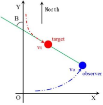
Figure 1. Motion Characteristics of Underwater Vehicle Approaching the Observer.
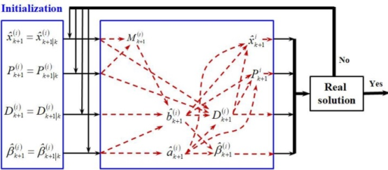
Figure 2.
A Fixed Point Iterative Scheme for Measurement Update Parameter Determination.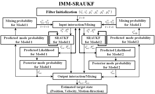
Figure 3. Schematic Diagram of IMM-SRAUKF Algorithm.
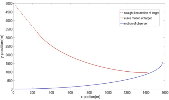
Figure 4. Target Motion to the Observer's Motion.
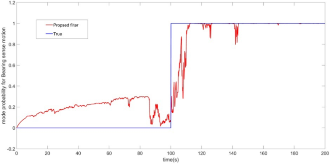
Figure 5. Mode Probabilities for Constant Velocity Models.
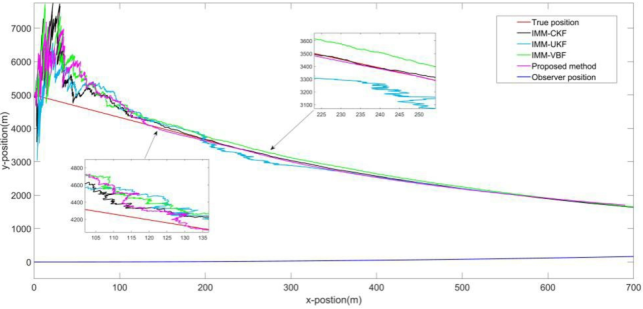
Figure 6. Comparison with Various Methods for Target Tracking.
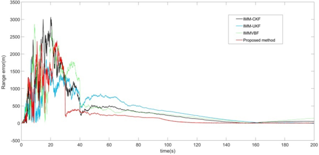
Figure 7. Comparison of Range Measurement Error of Various Methods for Target Tracking.


 and
and  is approximated as follows.
  in Eqs. (
 using Eqs. (
 using Eqs. (