Parameter Identification of Fractional-order Systems with Unknown Both State and Input Delays Based on Block Pulse Functions

Yu-Gang Hyon; Hyon-Ju Sin; Myong-Hyok Sin; Chol Min Sin; Hun Kim

doi:doi:10.11648/j.engmath.20250902.12

Research Article |

| Peer-Reviewed

Parameter Identification of Fractional-order Systems with Unknown Both State and Input Delays Based on Block Pulse Functions

Yu-Gang Hyon, Hyon-Ju Sin, Myong-Hyok Sin^*

, Chol Min Sin

, Hun Kim

Published in Engineering Mathematics (Volume 9, Issue 2)

Received: 27 October 2025 Accepted: 22 November 2025 Published: 29 December 2025

Views: Downloads:

Download PDF

Share This Article

Twitter
Linked In
Facebook

Abstract

In this paper, we propose a method for identification of continuous-time fractional-order systems with unknown states and input delays. In practice, many systems are modeled accurately with fractional differential equations. In particular, many systems are modeled as fractional differential equations with input delay and state delay. Since the geometric and physical meaning of fractional calculus is not clear, it is difficult to model the real system directly to fractional order systems based on mechanical analysis. Thus, the identification of fractional order systems is the main method for constructing fractional order models and is the subject of the main research by many scientists. To solve the identification problem of systems with input delay and state delay, we use the fact that the fractional integral operator matrix by the block pulse functions is an upper triangular Toeplitz matrix. We have presented an efficient method to identify the linear and nonlinear parameters separably by using the commutativity and nilpotent property for multiplication between upper triangular Toeplitz matrices. We also have presented an efficient algorithm to newly approximate the Jacobian of the variable projection functional to solve the least squares problem with nonlinear parameters. Several simulation examples have been used to verify the effectiveness of the proposed method. It is shown that the input delay and the state delay have a significant effect on the output characteristics of the system, especially the state delay has a larger effect than the input delay.

Published in	Engineering Mathematics (Volume 9, Issue 2)
DOI	10.11648/j.engmath.20250902.12
Page(s)	31-44
Creative Commons	This is an Open Access article, distributed under the terms of the Creative Commons Attribution 4.0 International License (http://creativecommons.org/licenses/by/4.0/), which permits unrestricted use, distribution and reproduction in any medium or format, provided the original work is properly cited.
Copyright	Copyright © The Author(s), 2025. Published by Science Publishing Group

Keywords

Block Pulse Function, Delay, Fractional Order System, Operational Matrix, Parameter Identification

1. Introduction

Due to non-local and historical memory properties of fractional order system (FOS), it has been widely studied by many researchers, see

[1-7]

. See also books

[8-10]

The time delay is one of the natural problem in the practical engineering applications. FOSs with time delays can be found in various engineering systems such as chemical process, nuclear reactor, and the dynamic behavior of HIV infection of

C D^{+}

T-cells, see

[11]

. In practice, FOSs with state delays arise from the dynamic behavior of viscoelastic materials, dynamical processes in self-similar and porous structures, control theory of mechanical system, strongly porous materials, some amorphous semiconductors, see

[12-18]

. In particular, they arise from communication lags, feedback delay in measurement, delay in closed loop systems. In

[17]

, the authors studied the control problem of SISO system which is presented as FOS with state delay when there exists a time delay in the state feedback loop. In

[18]

, the authors use the control signal composed of state delay signals to stabilize the vibration system of single degree of freedom. The stabilization of FOSs is greatly affected by state delay, see

[13, 16]

. So this is an important non-negligible factor in the construction of model for FOS with state delay.

Because of the lack of acceptable geometric or physical explanations of fractional calculus, the identification for FOSs has been the best approach for building fractional order models of physical systems.

It is well known that the time domain identification method is one of the identifications of FOSs. This is based on the minimization of both equation error and output error and hence several least square algorithms have been used. For example, we refer to a recursive error prediction approach

[19]

, modulating function method

[20, 21]

, Haar wavelet-based method

[22, 23]

, Block pulse functions (BPFs)-based method

[11, 24-28]

Due to the simplicity of BPFs, the identification method using BPFs has been considered as an effective one to avoid the complicated and costly computations of the fractional derivatives of input and output signals.

[11]

, to identify FOS with input delay, the fmincon function in MATLAB optimization toolbox was used to solve the optimization problem for determining both linear and nonlinear parameters. In the paper, the identification accuracy is sensitively varied according to the change of initial value. In general, the identification method for the linear continuous FOS which can estimate the linear and nonlinear parameters individually is considered as an efficient one having the independence of identification accuracy to initial condition and reducing the amount of work. In the context, we proposed an efficient identification method for FOS with both nonzero initial value and time delay, in which the linear and nonlinear parameters are individually estimated

[28]

Within our knowledge, for FOSs with state delay there seems to be no work concerning parameter identification method in which linear and nonlinear parameters are individually estimated. So the aim of this paper is to develop such an identification method for FOSs with unknown state and input delays. The main novelty is to derive a new method, by which the linear and nonlinear parameters are separably estimated by using the commutativity and nilpotent property of the fractional integral operational matrix (FIOM) of BPFs. Moreover, we propose an efficient algorithm based on a new approximation about the Jacobian of variable projection functional for solving the least squares method for nonlinear parameters. With the estimated nonlinear parameters, we use the bias compensated recursive least squares (BCRLS) method in order to reduce the amount of work and get a high accuracy in the identification of linear parameters.

Simulation results show that in the proposed methods the unknown state and input delays, coefficients are efficiently identified.

The paper consists of 5 sections. In section 2, we give the definitions of fractional calculus, BPFs and explain the commutativity and nilpotent property of the FIOM of BPFs, which is upper triangular Toeplitz. Section 3 is devoted to construction of a separable recursive model for FOSs with unknown state and input delays, and of a method in which the least square problem including all parameters is projected onto the one only including nonlinear parameters, i.e., state and input delays. In section 4, we give some simulation examples for verifying the effectiveness of the proposed method. Section 5 concludes this paper.

2. Preliminaries

2.1. Definitions of the Fractional Order Integral and Derivative

The Riemann-Liouville fractional order integral is defined by

_{t_{0}}^{R} I_{t}^{α} f (t) ≔ \frac{1}{Γ (α)} \int_{t_{0}}^{t} ‍ (t - s)^{α - 1} f (s) ds,

(1)

where

α > 0

(t_{0}, t)

is the integral interval and

Γ (\cdot)

is the Gamma function, that is,

Γ (α) : = \int_{0}^{\infty} ‍ x^{α - 1} e^{- x} dx

For the sake of simplicity, we set

t_{0} = 0

and denote

_{t_{0}}^{R} I_{t}^{α}

I^{α}

Let

l \in N, l - 1 < α < l

. Then the Riemann-Liouville fractional order derivative is defined as

\begin{matrix} D^{α} f (t) & = I^{- α} f (t) = D^{l} I^{l} I^{- α} f (t) = D^{l} I^{l - α} f (t) \\ = \frac{d^{l}}{d t^{l}} [\frac{1}{Γ (l - α)} \int_{t_{0}}^{t} ‍ (t - s)^{- α + l - 1} f (s) ds] . \end{matrix}

(2)

2.2. The FIOM of BPFs

As in

[29]

, a set of BPFs in the semi-open interval

[0, T)

is defined by

B_{n} (t) : = \{\begin{matrix} 1, \frac{n - 1}{N} T \leq t < \frac{n}{N} T, \\ 0, otherwise, \end{matrix}

(3)

where

n = 1, \dots, N

, and

N

is the number of BPFs in the set.

We call

B (t) : = [B_{1} (t), \dots, B_{N} (t)]^{T}

by block pulse vector. If we define the elements of

X = [x_{1}, . . ., x_{N}]^{T}

x_{n} = \frac{N}{T} \int_{\frac{n - 1}{N} T}^{\frac{n}{N} T} ‍ x (t) dt \approx x (\frac{n - 1}{N} T),

then any absolute integrable function defined on interval

[0, T)

can be approximated by a linear combination of BPFs as follow:

x (t) = \sum_{n = 1}^{N} ‍ [\frac{N}{T} \int_{\frac{n - 1}{N} T}^{\frac{n}{N} T} ‍ x (t) dt] B_{n} (t) \approx \sum_{n = 1}^{N} ‍ x_{n} B_{n} (t) = X^{T} B (t) .

(4)

By Eq. (1), we have

I^{α} B (t) = \frac{1}{Γ (α)} t^{α - 1} * B (t),

(5)

where the symbol

*

means convolution. In

[30]

, it was shown that Eq. (5) can be represented as

I^{α} B (t) \approx P_{α} B (t),

(6)

where

P_{α} : = \frac{h^{α}}{Γ (α + 2)} (\begin{matrix} ξ_{1} & ξ_{2} & ξ_{3} & \dots & ξ_{N} \\ 0 & ξ_{1} & ξ_{2} & \dots & ξ_{N - 1} \\ 0 & 0 & ξ_{1} & \dots & ξ_{N - 2} \\ \dots & \dots & \dots & \dots & \dots \\ 0 & 0 & 0 & 0 & ξ_{1} \end{matrix}),

(7)

h = \frac{T}{N}, ξ_{1} = 1, ξ_{l} = l^{α + 1} - 2 (l - 1)^{α + 1} + (l - 2)^{α + 1}, l = 2, . . ., N .

We call the matrix

P_{α}

by FIOM for BPFs. By Eqs. (4), (6), the fractional order integral of the function

x (t)

is given by

I^{α} x (t) \approx X^{T} P_{α} B (t) .

(8)

2.3. Commutativity and Nilpotent Property of the FIOM

By Eq. (4), the function

x (t - τ)

is expanded by BPFs as follow:

x (t - τ) \approx X^{T} B (t - τ) = \sum_{i = 1}^{N} ‍ x_{i} B_{i} (t - τ),

(9)

where

x_{i} = \frac{1}{h} \int_{0}^{T} ‍ x (t - τ) B_{i} (t - τ) dt .

(10)

[11]

, it was pointed out that for

τ = kh

, the delayed function

B (t - τ)

is represented as

B (t - τ) = E_{k} \cdot B (t), t > τ, 0 \leq t \leq T,

(11)

where for the Kronecker delta function

δ_{ij}

E_{k} = {(δ_{i, j + k})}_{i, j = 1}^{n}, k = 0, 1, \dots, n - 1 .

(12)

The matrix

E_{k}

is called

k

order delay operational one. In

[28]

, it was shown that for non-negative integers

i, j

E_{i} E_{j} = E_{j} E_{i} = \{\begin{matrix} I, if i + j = 0 \\ E_{i + j}, if i + j < N \\ 0, if i + j \geq N . \end{matrix}

(13)

As in

[11]

, the Riemann-Liouville fractional order integral

B (t - τ)

is rewritten as

(I^{α} B) (t - τ) \approx P_{α} B (t - τ) = P_{α} E_{k} B (t) .

(14)

By Eq. (12), the FIOM from Eq. (7) is decomposed into

P_{α} = \sum_{i = 0}^{N - 1} ‍ \frac{h^{α}}{Γ (α + 2)} ξ_{i + 1} E_{i} .

(15)

From Eq. (15), we can see that the FIOM from Eq. (7) is upper triangular Toeplitz which belongs to the subspace

T_{N} = Span \{E_{0}, E_{1}, \dots, E_{N - 1}\}

Next, let us consider the commutativity of FIOMs. In the Appendix A below, we show the following properties: for any two FIOMs,

A, B \in T_{N}

and

i, j = 0, 1, 2, \dots

\begin{matrix} i) A^{i} B^{j} \in T_{N}, \\ ii) A^{i} B^{j} = B^{j} A^{i}, \\ iii) {(AB)}^{i} = A^{i} B^{i} . \end{matrix}

(16)

[31]

, it was shown that if a matrix

A

belongs to the strict upper triangular Toeplitz space

S T_{N} = Span \{E_{1}, \dots, E_{N - 1}\}

, then

A

is nilpotent. Indeed, if

A \in S T_{N}

, then by (13) for all

k (\geq N)

A^{k} = 0 .

(17)

Remark 1 Eq. (17) is the main key in the transformation of identification of FOS with state delay onto the separable least square problem. In particular, by Eqs. (16) and (17), we get that for

B = \sum_{k = 0}^{N - 1} ‍ b_{k + 1} E_{k} \in T_{N}

and

Q = \sum_{k = 1}^{N - 1} ‍ b_{k + 1} E_{k}

B^{- 1} = {(b_{1} I + Q)}^{- 1} = \sum_{k = 0}^{N - 1} ‍ \frac{Q^{k}}{{(- b_{1})}^{k + 1}} .

(18)

For more detail, we refer to Appendix B.

3. Identification Algorithm for FOSs with Unknown State and Input Delays

Here we construct a new identification algorithm for FOSs with unknown state and input delays using separable least square problem. At first, the identification method is proposed for FOS from

[14]

and then for FOS from

[12, 13, 16]

3.1. Case 1

Let us consider the FOS from

[14]

\begin{matrix} D^{α} x (t) + ax (t - τ_{a}) = bu (t - τ_{b}), \\ y (t) = x (t) + w (t), \end{matrix}

(19)

where

τ_{a} = kh, τ_{b} = lh

and

N

is the number of BPFs and

T

is the simulation time, and

u (t)

x (t)

y (t)

w (t)

are input signal, state, output signal and the Gauss white noise, respectively.

From Eqs. (8) and (14) the first equation in Eq. (19) can be rewritten as

X^{T} (I + a P_{α} E_{k}) B (t) = b U^{T} P_{α} E_{l} B (t) .

Hence by (4)

x (t) = b U^{T} P_{α} E_{l} {(I + a P_{α} E_{k})}^{- 1} B (t) .

(20)

By Eq. (18), the matrix

{(I + a P^{α} E_{k})}^{- 1}

with

k \geq 1

is the following:

{(I + a P_{α} E_{k})}^{- 1} = \sum_{i = 0}^{N - 1} ‍ {(- 1)}^{i} a^{i} P_{α}^{i} E_{ki} .

(21)

Inserting Eq. (21) into Eq. (20) implies that

x (t) = b U^{T} P_{α} E_{l} [\sum_{i = 0}^{N - 1} ‍ {(- 1)}^{i} a^{i} P_{α}^{i} E_{ki}] B (t) .

(22)

Now we set

θ_L = (θ_1, θ_2, \dots, θ_N)^T, θ_i = (- 1)^(i - 1) ba^(i - 1), θ_NL = (k, l)^T,

φ (θ_NL, t) = (█ (U^T P_α E_l B (t), U^T P_α^2 E_(k + l) B (t), U^T P_α^3 E_(2 k + l) B (t), \dots @, U^T P_α^N E_((N - 1) k + l) B (t)))_(1 \times N) .

Mk + l < N \leq (M + 1) k + l

, then by the previous notation Eq. (22) can be rewritten as

x (t) = φ (θ_{NL}, t) θ_{L},

(23)

where

φ (θ_NL, t) = (U^T P_α E_l B (t), U^T P_α^2 E_(k + l) B (t), \dots, U^T P_α^(M + 1) E_(Mk + l) B (t), 0, \dots, 0) .

(24)

Remark 2 In the estimation of the nonlinear parameter

θ_{NL} = {(k, l)}^{T}

, for

τ_{a}, τ_{b} \in [τ_{\min}, τ_{\max}]

k, l \in [i_{\min}, i_{\max}]

, only the first up to

M + 1 = [N / i_{\min}]

elements in Eq. (24) can be non-zero. The greater

k

and

l

, the smaller the amount of work.

By Eq. (24) the data matrix

Φ (θ_{NL})

for

N

sampling points can be written as

Φ (θ_{NL}) = {\{φ_{ij} (θ_{NL})\}}_{N \times N},

(25)

where

φ_{ij} (θ_{NL}) = \{\begin{matrix} U^{T} P_{α}^{j} E_{(j - 1) k + l} B (i), if i = 1, \dots, N, j = 1, \dots, M + 1, \\ 0, if j > M + 1 . \end{matrix}

(26)

Then by Eqs. (25) and (26) the identification for (19) is reduced to the separable least square problem as

R (θ_{L}, θ_{NL}) = {‖Y - Φ (θ_{NL}) θ_{L}‖}_{2}^{2} : \min,

(27)

where

Y

is sampling value vector for

y (t)

3.2. Case 2

Let us consider the FOS from

[12, 13, 16]

\begin{matrix} D^{α} x (t) + a_{1} x (t - τ_{a}) + a_{0} x (t) = bu (t - τ_{b}), \\ y (t) = x (t) + w (t), \end{matrix}

(28)

where

τ_{a} = kh, τ_{b} = lh

N

T

u (t), x (t), y (t), w (t)

are the same as in the FOS (19).

From Eq. (8) we can rewrite Eq. (28) as

X^{T} (I + a_{1} P_{α} E_{k} + a_{0} P_{α}) B (t) = b U^{T} P_{α} E_{l} B (t) .

Hence

x (t) = b U^{T} P_{α} E_{l} {(I + a_{1} P_{α} E_{k} + a_{0} P_{α})}^{- 1} B (t) .

(29)

From (18) and Appendix C, the matrix

{(I + a_{1} P^{α} E_{k} + a_{0} P_{α})}^{- 1}

with

k \geq 1

can be rewritten as

{(I + a_{1} P_{α} E_{k} + a_{0} P_{α})}^{- 1} = \sum_{n = 0}^{N - 1} ‍ c_{1} c_{2}^{n} D_{α} (c_{3}, k, n),

(30)

where

c_{1} : = \frac{1}{1 + a_{0} f_{1}}, c_{2} : = \frac{a_{1}}{1 + a_{0} f_{1}}, c_{3} : = \frac{a_{0}}{a_{1}}, D_{α} (c_{3}, k, n) : = \sum_{i = 0}^{n} ‍ c_{3}^{n - i} E_{ik} S_{α} (n, i)

. Once

α

is known, the matrix

S_{α} (n, i)

is represented as

S_{α} (n, i) = (\begin{matrix} n \\ i \end{matrix}) P_{α}^{i} {(P_{α} - (α + 2) ξ_{1} I)}^{n - i} .

Remark 3 If

|c_{3}| \leq 1

, then the convergence of proposed algorithm is guaranteed with increase of the number of BPFs. If

|c_{3}| > 1

, then in Appendix C we can set

a_{1} / a_{0} = c_{3}

and modify the algorithm.

Inserting (30) into (29) implies that

x (t) = b U^{T} P_{α} E_{l} \sum_{n = 0}^{N - 1} ‍ {(- 1)}^{n} c_{1} c_{2}^{n} D_{α} (c_{3}, k, n) B (t) .

(31)

θ_{n} = {(- 1)}^{n} b c_{1} c_{2}^{n}, n = 0, 1, \dots, N - 1

, in Eq. (31), then

θ_{L} = {(θ_{0}, θ_{1}, \dots, θ_{N - 1})}^{T}

is the linear parameter and

θ_{NL} = {(c_{3}, k, l)}^{T}

the nonlinear parameter. Then Eq. (31) can be rewritten as

x (t) = φ (θ_{NL}, t) θ_{L},

(32)

where

■ (φ (θ_NL, t) = (U^T P_α E_l D_α (c_3, k, 0) B (t), \dots,

U^T P_α E_l D_α (c_3, k, n) B (t), @ \dots,

U^T P_α E_l D_α (c_3, k, N - 1) B (t)) .)

(33)

By Eq. (32) the data matrix

Φ (θ_{NL})

for

N

sampling points can be rewritten as

Φ (θ_{NL}) = {\{φ_{ij} (θ_{NL})\}}_{N \times N},

(34)

where

φ_{ij} (θ_{NL}) = U^{T} P_{α} E_{l} D_{α} (c_{3}, k, j - 1) B (i), i, j = 1, \dots, N .

(35)

Thus from Eqs. (31) and (34) the identification for the FOS (28) is reduced to the separable least square problem

R (θ_{L}, θ_{NL}) = {‖Y - Φ (θ_{NL}) θ_{L}‖}_{2}^{2} : \min,

(36)

where

Y

is the sampling value vector of

y (t)

3.3. Identification Algorithm

3.3.1. Identification Algorithm for Nonlinear Parameter

As we can see in Eqs. (27) and (36), the identifications for FOSs (19) and (28) with both state and input delays are reduced to the separable least square problem.

[32]

, given the nonlinear parameter

θ_{NL}

, the solution of the optimization problem (27) and (36) for obtaining the linear parameters is

θ_{L} = Φ^{+} (θ_{NL}) Y,

(37)

where

Φ^{+} (θ_{NL}) = {[Φ^{T} (θ_{NL}) Φ (θ_{NL})]}^{- 1} Φ^{T} (θ_{NL})

is Moore-Penrose pseudo-inverse.

Inserting Eq. (37) into Eq. (27) or (36) yields that we have the following optimization for nonlinear parameter

θ_{NL}

R_{1} (θ_{NL}) = {‖(I - P (θ_{NL})) Y‖}^{2} : \min,

(38)

where

P (θ_{NL}) = Φ (θ_{NL}) Φ^{+} (θ_{NL}) \in R^{N \times N}

and

f (θ_{NL}) : = (I - P (θ_{NL})) Y

(39)

is a variable projection functional.

The matrix

Φ^{+} (θ_{NL})

needs the inverse matrix

{[Φ^{T} (θ_{NL}) Φ (θ_{NL})]}^{- 1}

. However, the matrix

Φ^{T} (θ_{NL}) Φ (θ_{NL})

can be singular. To solve the problem, we follow the argument from

[28]

If the matrix

Φ^{-} (θ_{NL})

satisfies

Φ (θ_{NL}) Φ^{-} (θ_{NL}) Φ (θ_{NL}) = Φ (θ_{NL}), {(Φ (θ_{NL}) Φ^{-} (θ_{NL}))}^{T} = Φ (θ_{NL}) Φ^{-} (θ_{NL}),

(40)

then the matrix

P (θ_{N L})

from (38) can be rewritten as

P (θ_{NL}) = Φ (θ_{NL}) Φ^{-} (θ_{NL}) .

(41)

Here the matrix

Φ^{-} (θ_{NL})

can be obtained as follow: if

r ank Φ (θ_{NL}) = r

, then the matrix

Φ (θ_{NL})

is decomposed as

Φ (θ_{NL}) = G (\begin{matrix} U_{11} & U_{12} \\ 0 & 0 \end{matrix}),

(42)

where

r ank U_{11} = r, U_{11} \in R^{r \times r}

and

U_{11}

has normally orthonormal column vectors. Then the matrix

Φ^{-} (θ_{NL}) = (\begin{matrix} U_{11}^{- 1} & 0 \\ 0 & 0 \end{matrix}) G^{T}

satisfies Eq. (40). Setting

G = [G_{1}, G_{2}], G_{1} \in R^{N \times r}

, we have

P (θ_{NL}) = G_{1} G_{1}^{T} .

(43)

Thus Eq. (38) is represented as

R_{2} (k) = {‖(I - G_{1} G_{1}^{T}) Y‖}^{2} : \min .

(44)

As pointed out in

[28]

, the matrix

G_{1}

consists of the first linear independent

r

column vectors which are obtained by orthonormalizing

Φ (θ_{NL})

by virtue of Gram-Schmidt orthogonalization.

In order to identify the nonlinear parameter based on Levenberg-Marquardt (LM) algorithm from

[31]

, we have to construct the Jacobian for the cost functional (44).

Remark 4 In this paper, we propose a new construction of Jacobian of variable projection functional, in which the matrix

Φ^{+}

is no longer used.

To this end, we first calculate the Jacobian of variable projection functional

f (θ_{NL})

from (39). If

θ_{NL} = {(x_{1}, x_{2}, \dots, x_{m})}^{T}

for

m = 2

or 3, then we have for

k = 1, \dots, m

■ (\nabla_k f = - (\nabla_k Φ) Φ^+ Y + Φ [\nabla_k (Φ^+)] Y = - (\nabla_k Φ) Φ^+ Y + Φ \nabla_k [(Φ^T Φ)^(- 1) Φ^T] Y @ = - (\nabla_k Φ) Φ^+ Y + Φ (Φ^T Φ)^(- 1) [(\nabla_k Φ)^T Φ - Φ^T (\nabla_k Φ)] (Φ^T Φ)^(- 1) Φ^T Y @ = - [\nabla_k Φ + (Φ^+)^T (\nabla_k Φ)^T Φ - ΦΦ^+ (\nabla_k Φ)] Φ^+ Y .)

[33]

we can neglect the term

{(Φ^{+})}^{T} {(\nabla_{k} Φ)}^{T} Φ Φ^{+} Y

in the previous formula. This enables us to reduce the amount of work without a great affection about the approximation accuracy of Jacobian. By (43) we have

\begin{matrix} \nabla_{k} f \approx - [\nabla_{k} Φ - Φ Φ^{+} (\nabla_{k} Φ)] Φ^{+} Y = - (I - Φ Φ^{+}) (\nabla_{k} Φ) Φ^{+} Y \\ = - (I - G_{1} G_{1}^{T}) (\nabla_{k} Φ) Φ^{+} Y . \end{matrix}

(45)

Since

Φ^{+} Y = Φ^{+} Φ θ_{L} = Φ^{+} Φ Φ^{-} Φ θ_{L} = Φ^{-} Y

by (40) and (41), we have

\nabla_{k} f \approx - (I - G_{1} G_{1}^{T}) (\nabla_{k} Φ) Φ^{-} Y .

(46)

Moreover,

{(\nabla_{k} Φ)}_{ij}, i, j = 1, \dots, N,

can be obtained as follow: for the case 1 with

x_{1} = k, x_{2} = l

\begin{matrix} {(\nabla_{1} Φ)}_{ij} \approx U^{T} P_{α}^{2} E_{(j - 1) (k + 1) + l} B (i) - U^{T} P_{α}^{2} E_{(j - 1) k + l} B (i), \\ {(\nabla_{2} Φ)}_{ij} \approx U^{T} P_{α}^{2} E_{(j - 1) k + l + 1} B (i) - U^{T} P_{α}^{2} E_{(j - 1) k + l} B (i), \end{matrix}

(47)

while for the case 2 with

x_{1} = c_{3}, x_{2} = k, x_{3} = l

■ ((\nabla_1 Φ)_ij = U^T P_α E_l \partial / (\partial c_3) D_α (c_3, k, j - 1) B (i), @ (\nabla_2 Φ)_ij \approx U^T P_α E_l D_α (c_3, k + 1, j - 1) B (i) - U^T P_α E_l D_α (c_3, k, j - 1) B (i), @ (\nabla_3 Φ)_ij \approx U^T P_α E_(l + 1) D_α (c_3, k, j - 1) B (i) - U^T P_α E_l D_α (c_3, k, j - 1) B (i),)

(48)

where

\frac{\partial}{\partial c_{3}} D_{α} (c_{3}, k, j - 1) = \sum_{l = 0}^{j - 1} ‍ (j - 2 - l) c_{3}^{j - 2 - l} E_{lk} S_{α} (j - 1, l) .

By Eqs. (47) and (48) the algorithm for determining the nonlinear parameter

θ_{NL}

is constructed as follow:

[Algorithm 1]

Step 1: Set

k = 0

and select the initial point

θ_{NL} (0)

and admissible error

ε > 0

Step 2: Set

θ_{NL} (k + 1) = θ_{NL} (k) + λ_{k} d_{k}

and determine the scrutiny direction

d_{k}

[J {(θ_{NL} (k))}^{T} J (θ_{NL} (k)) + λ_{k} I] d_{k} = - J (θ_{NL} (k)) E (θ_{NL} (k)),

where

E = (I - G_{1} G_{1}^{T}) Y

is error function,

λ_{k}

damping factor. The Jacobian

J (θ_{NL} (k))

is determined by Eq. (45) as

J (θ_{NL} (k)) = (\begin{matrix} \nabla_{1} f (θ_{NL} (k)), & \nabla_{2} f (θ_{NL} (k)), & \dots, & \nabla_{m} f (θ_{NL} (k)) \end{matrix}),

where

m = 2

for the case 1, while

m = 3

for the case 3. The step size

λ_{k}

is determined by

\underset{λ \geq 0}{argmin} {‖(I - P (θ_{NL} (k) + λ d_{k})) Y‖}^{2}

Step 3: If

{‖(I - P (θ_{NL} (k + 1))) Y‖}^{2} < ε

, then we set

{\hat{θ}}_{NL} = θ_{NL} (k + 1)

and if not, then go to step 2 with

k = k + 1

3.3.2. Identification Algorithm for Linear Parameters

If the nonlinear parameter

θ_{NL}

is estimated by algorithm 1, the linear parameter

θ_{L}

can be estimated by Eq. (37).

Remark 5 As mentioned above, the matrix

Φ^{+} (θ_{NL})

does not exist if

\det [Φ^{T} (θ_{NL}) Φ (θ_{NL})] = 0

. Moreover, it is pointed out in

[25]

that even though

\det [Φ^{T} (θ_{NL}) Φ (θ_{NL})] \neq 0

, the linear parameter estimated by Eq. (37) has a deviation when there exists an output noise. Furthermore, increase of the number of BPFs yields increase of the number of the linear parameters, which makes it impossible for us to calculate them. Hence we use BCRLS method from

[25]

We select

t = (p - 1) h, p = 1, . . ., N,

as sampling times and introduce the notations

X^{T} B (t) = X_{1} (p), X^{T} P_{α} B (t) = X_{0} (p), U^{T} P_{α} B (t) = U_{0} (p) .

(49)

Then the FOS (19) or (28) can be rewritten as

X_{1} (p) = φ (p, \hat{k}, \hat{l}) θ_{L},

(50)

where

\hat{k}, \hat{l}

are the already estimated nonlinear parameters.

For the FOS (19), we have

\begin{matrix} φ (p, \hat{k}, \hat{l}) = [- X_{0} (p - \hat{k}), U_{0} (p - \hat{l})], for p = 1, \dots, N \\ θ_{L} = {(a, b)}^{T}, \end{matrix}

(51)

and while for the FOS (28)

\begin{matrix} φ (p, \hat{k}, \hat{l}) = [- X_{0} (p - \hat{k}), - X_{0} (p), U_{0} (p - \hat{l})], for p = 1, \dots, N \\ θ_{L} = {(a_{1}, a_{0}, b)}^{T} . \end{matrix}

(52)

Then the BCRLS for estimating linear parameters is the following:

[Algorithm 2]

■ (L (p, k ̂, l ̂) = Q (p - 1) φ (p, k ̂, l ̂) [λ + φ^T (p, k ̂, l ̂) Q (p - 1) φ (p, k ̂, l ̂)]^(- 1), Q (0) = p_0 I, @ ε (p, k ̂, l ̂) = y (p) - φ ̂^T (p, k ̂, l ̂) θ ̂_RLS (p - 1), @ θ ̂_RLS (p, k ̂, l ̂) = θ ̂_RLS (p - 1, k ̂, l ̂) + L (p, k ̂, l ̂) ε (p, k ̂, l ̂), @ Q (p, k ̂, l) = [I - L (p, k ̂, l ̂) φ^T (p, k ̂, l ̂)] Q (p - 1, k ̂) / λ, @ θ_BCRLS (p, k ̂, l ̂) = θ_RLS (p - 1, k ̂, l ̂) @ - Q (p, k ̂, l ̂) [\sum_(i = 1)^t ▒‍ φ (i, k ̂, l ̂) (X_n (i) - φ^T (i, k ̂, l ̂) θ_RLS (i, k ̂, l ̂))],)

(53)

where

Q (0) = γI, {\hat{θ}}_{RLS} (0) = {(1 / p_{0}, \dots, 1 / p_{0})}^{T}

and

γ

is a very large parameter which usually has the size of

(1 0^{3} : 1 0^{8})

and

0.2 \leq λ < 1

4. Simulation Examples

Example 1

We consider

\begin{matrix} D^{α} x (t) + ax (t - τ_{a}) = bu (t - τ_{b}), \\ y (t) = x (t) + w (t), \end{matrix}

(54)

where

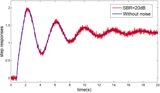
a = 1.1, b = 1.5, τ_{a} = 1.2, τ_{b} = 0.8, α = 0.7

and

w (t)

is the Gauss white noise. The simulation time is

T = 20 s

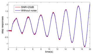
Figure 1 shows the step response for the FOS (54) with noise or without noise.

Download: Download full-size image

Figure 1. The Step Response for Example 1.

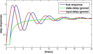
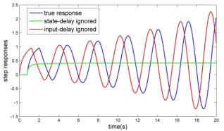
To show the dependence of output response to input or state delays, we present Figure 2.

Download: Download full-size image

Figure 2. The Step Response for Example 1 with Ignored State or Input Delay.

As we can see in Figure 2, the output response for the system with ignored state delay is greatly different from real response than the one for the system with ignored input delay. This shows that the state delay is an important non-negligible factor.

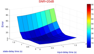
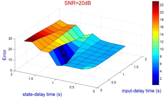
Figure 3 shows the error function (44) for the FOS (54) without noise or with noise

SNR = 20 dB

, in which the errors for state delay

τ_{a}

and input delay

τ_{b}

is presented in the range of

[0.2, 1.6]

(a) Without Noise. (b) with Noise.

Download: Download full-size image

Figure 3. The Error Function for FOS (54).

Table 1 lists the identification results of nonlinear parameters

τ_{a}, τ_{b}

for the FOS (51) with noise or without noise. Here the algorithm 1 is used.

Table 1. Identification Results of Nonlinear Parameters for Example 1.

nonlinear parameter	true(s)	without noise	with noise (SNR)
nonlinear parameter	true(s)	without noise	10dB	20dB
state delay time	1.2	1.2000	1.2000	1.2000
input delay time	0.8	0.8000	0.8000	0.8000

Table 1 shows that if the state and input delay times are integer times of the sampling interval

T / N

, then there does not exist the identification error for nonlinear parameters.

Based on this identification result, we can estimate the linear parameters. Here we use algorithm 2.

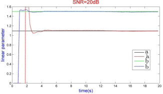
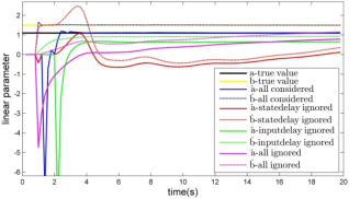
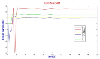
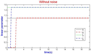
In Figure 4, the online identification process of linear parameters for the FOS (54) with noise or without noise is presented.

(a) Without Noise (b) with Noise

Download: Download full-size image

Figure 4. The Identification Result for FOS (54).

Table 2 shows the identification result according to various noise and numbers of BPFs. Table 2 represents the average values of 50 identification results obtained by using Monte-Carlo methods. In Table 2, we present the identification accuracy by the relative error between real parameter

θ = {(a, b)}^{T}

and estimated one

\hat{θ} = {(\hat{a}, \hat{b})}^{T}

, i.e.,

δ = \frac{‖θ - \hat{θ}‖}{‖θ‖} \times 100 (%) .

(55)

Table 2. The Identification Result According to Various Noise and Numbers of BPFs.

linear parameter	true	BPFs' number =100			BPFs' number =500
linear parameter	true	SNR=10dB	SNR=20dB	SNR=50dB	SNR=10dB	SNR=20dB	SNR=50dB
$a$	1.1	1.1313	1.0898	1.1001	1.0986	1.0998	1.1000
$b$	1.5	1.6241	1.4997	1.4999	1.5014	1.5001	1.5000
$δ$	-	6.88	0.54	7.6e-03	0.100	0.010	0.000

From Table 2, we can see that the more increase the number of BPFs, the more improve the identification accuracy.

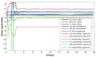
Figure 5 shows the online identification process of example 1 with ignored state delay or input delay. Here

SNR = 20 dB

and

N = 100

Download: Download full-size image

Figure 5. The Dependence of Online Identification for Linear Parameters to Nonlinear Parameters.

Download: Download full-size image

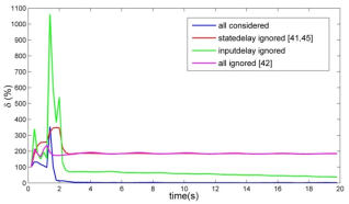
Figure 6. The Dependence of Error Function to Nonlinear Parameters.

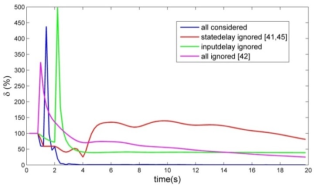
In order to analyse the identification accuracy in more detail, we present the dependence of the function (55) to the nonlinear parameters, see Figure 6. Figure 6 shows that for FOS with both state and input delays, identification result of linear parameters is greatly different from the one for FOS with only input delay

[11, 28]

, and without any delay

[25]

. In particular, the identification result is worse for FOS without state delay.

Example 2

We consider the system

\begin{matrix} D^{α} x (t) + a_{1} x (t - τ_{a}) + a_{0} x (t) = bu (t - τ_{b}), \\ y (t) = x (t) + w (t), \end{matrix}

(56)

where

a_{1} = 2.5, a_{0} =, b = 1 . . 5, τ_{a} = 1.2, τ_{b} = 0.8, α = 0.7

w (t)

is the Gauss white noise and

T = 20 s

Figure 7 shows the step response for the FOS (56) with noise or without noise.

Download: Download full-size image

Figure 7. The Step Response for Example 2.

To show the dependence of output response to input or state delays, we present Figure 8.

Download: Download full-size image

Figure 8. The Step Response for Example 2 with Ignored State or Input Delay.

As example 1, the output response for the system with ignored state delay is greatly different from real response than the one for the system with ignored input delay. This also shows that the state delay is an important non-negligible factor.

Figure 9 shows the error function (44) for the FOS (56) without noise or with noise

SNR = 20 dB

when

c_{3} = 0.25

. Here the errors for state delay

τ_{a}

and input delay

τ_{b}

is presented in the range of

[0.2, 1.6]

(a) Without Noise. (b) with Noise.

Download: Download full-size image

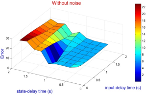
Figure 9. The Error Function for FOS (56).

From Figure 9 we can see that the error function (44) for the FOS (56) is seldom affected by the output noise.

Table 3 presents the identification results of nonlinear parameters

τ_{a}, τ_{b}

for the FOS (56) with noise or without noise.

Table 3. Identification Results of Nonlinear Parameters for the FOS(56).

nonlinear parameter	true(s)	without noise	with noise
nonlinear parameter	true(s)	without noise	SNR=10dB	SNR=20dB
state delay time	1.2	1.2000	1.2000	1.2000
input delay time	0.8	0.8000	0.8000	0.8000
auxiliary parameter	0.25	0.2500	0.2492	0.2501

Based on this identification result, we can estimate the linear parameters. Here we also use algorithm 2.

Figure 10 show the online identification process of linear parameters for the FOS (56) with noise or without noise.

(a) Without Noise (b) with Noise.

Download: Download full-size image

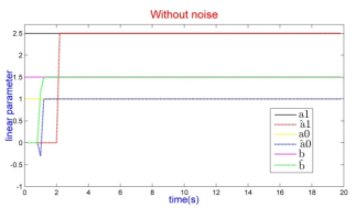
Figure 10. The Identification Result of Linear Parameters for FOS (56).

Table 4 lists the identification result according to various noise and numbers of BPFs by the average values of 50 identification results obtained by using Monte-Carlo methods.

Table 4. The Identification Result According to Various Noise and Numbers of BPFs.

linear parameter	true	BPFs' number =100			BPFs' number =500
linear parameter	true	SNR=10dB	SNR=20dB	SNR=50dB	SNR=10dB	SNR=20dB	SNR=50dB
$a_{1}$	2.5	2.3909	2.4872	2.4997	2.4984	2.4999	2.5000
$a_{0}$	1.0	0.9670	1.1012	1.0054	1.0007	1.0003	1.0002
$b$	1.5	1.6103	1.5136	1.5019	1.5012	1.5001	1.5000
$δ$	-	5.1460	3.3388	1.7531	0.0687	0.0107	0.0064

From Table 4, we can see that the more increase the number of BPFs, the more improve the identification accuracy. Figure 11 shows the online identification process of example 2 with ignored state delay or input delay. Here

SNR = 20 dB

and

N = 100

Download: Download full-size image

Figure 11. The Dependence of Online Identification of Linear Parameters to Nonlinear Parameters.

In Figure 12 the dependence of the function (55) to the nonlinear parameters is presented.

Download: Download full-size image

Figure 12. The Dependence of Error Function to Nonlinear Parameters.

From Figure 12 we can see that for linear continuous FOS, the identification accuracy of linear parameters is affected strongly by state delay than input delay and is nearly similar for the case of ignoring only state delay and the case of ignoring both state and input delay. Hence the state delay time must be estimated for linear continuous FOS with state delay.

5. Conclusion

In this paper, the identification method for linear continuous FOS with unknown state and input delays is proposed.

Simulation results show that the proposed method has a high identification accuracy for FOS with unknown state and input delays. In particular, Simulation result shows that the state delay is an important non-negligible factor.

Our further study is to develop an identification method for fractional order systems with unknown state and input delays, in which not only the delays and efficient but also differential order are estimated.

Abbreviations

FOS	Fractional Order System
BPF	Block Pulse Function
FIOM	Fractional Integral Operational Matrix
BCRLS	Bias Compensated Recursive Least Squares
LM	Levenberg-Marquardt

Author Contributions

Yu-Gang Hyon: Conceptualization, Writing – original draft

Hyon-Ju Sin: Data curation, Formal Analysis

Myong-Hyok Sin: Writing – original draft

Chol Min Sin: Data curation, Formal analysis, Writing – review & editing

Hun Kim: Validation, Software

Conflicts of Interest

The author declares no conflicts of interest.

Appendix

Appendix I: Proof of Eq. (16)

At first, let us prove i) in Eq. (16). Let

i = 2, j = 0

. Then

A^{2} \in T_{N} .

(57)

By Eq. (15) we have

A = \sum_{k = 0}^{N - 1} ‍ a_{k + 1} E_{k}

. Hence the matrix

A^{2}

is represented as

A^{2} = \sum_{p = 1}^{N - 1} ‍ \sum_{q = 1}^{N - 1} ‍ a_{p + 1} a_{q + 1} E_{p} E_{q} .

(58)

By Eq. (13), Eq. (58) can be rewritten as

A^{2} = \sum_{p = 0}^{N - 1} ‍ \sum_{q = 0}^{N - 1} ‍ a_{p + 1} a_{q + 1} E_{p + q} = \sum_{k = 0}^{N - 1} ‍ c_{k + 1} E_{k},

where

0 \leq k = p + q \leq N - 1

c_{k + 1} = \sum_{p = 0}^{k} ‍ a_{p + 1} a_{k - p + 1}

. Thus Eq. (57) holds.

For

i = 1, j = 1

, we can follow the same argument to get

AB \in T_{N},

(59)

where

AB = \sum_{p = 0}^{N - 1} ‍ \sum_{q = 0}^{N - 1} ‍ a_{p + 1} b_{q + 1} E_{p + q} = \sum_{k = 0}^{N - 1} ‍ d_{k + 1} E_{k}, d_{k + 1} = \sum_{p = 0}^{k} ‍ a_{p + 1} b_{k - p + 1} .

(60)

By Eqs. (57) and (59) we have

A^{i}, B^{j} \in T_{N}

and

A^{i} B^{j} \in T_{N}

It suffices to prove only

AB = BA

for verifying ii) in Eq. (16). That

AB = BA

is obvious by Eq. (60).

The validity of iii) in Eq. (16) follows immediately from ii).

Appendix II: Proof of Eq. (18)

Here we prove Eq. (18). We have

(b_{1} I + Q) \sum_{k = 0}^{N - 1} ‍ \frac{Q^{k}}{{(- b_{1})}^{k + 1}} = \sum_{k = 0}^{N - 1} ‍ \frac{Q^{k}}{{(- b_{1})}^{k}} + \sum_{k = 0}^{N - 1} ‍ \frac{Q^{k + 1}}{{(- b_{1})}^{k + 1}} = I + \frac{Q^{N}}{{(- b_{1})}^{N}} .

On the other hand,

Q^{N} = 0

by Eq. (17). Thus Eq. (18) is valid.

Appendix III: Proof of Eq. (30)

Here we prove Eq. (30). For simplicity, we set

f_{i} ≔ \frac{h^{α}}{Γ (α + 2)} ξ_{i}

. Direct calculations show that

■ ((I + a_1 P_α E_k + a_0 P_α)^(- 1) = (I + a_1 P_α E_k + a_0 f_1 I + a_0 \sum_(i = 1)^(N - 1) ▒‍ f_(i + 1) E_i)^(- 1) @ = ((1 + a_0 f_1) I + a_1 P_α E_k + a_0 \sum_(i = 1)^(N - 1) ▒‍ f_(i + 1) E_i)^(- 1) @ = 1 / (1 + a_0 f_1) (I + a_1 / (1 + a_0 f_1) P_α E_k + a_0 / (1 + a_0 f_1) \sum_(i = 1)^(N - 1) ▒‍ f_(i + 1) E_i)^(- 1) .)

Using the result from Appendix A, we have for

k \neq 0

{(I + a_{1} P_{α} E_{k} + a_{0} P_{α})}^{- 1} = \frac{1}{1 + a_{0} f_{1}} \sum_{n = 0}^{N - 1} ‍ {(- 1)}^{n} {(\frac{a_{1}}{1 + a_{0} f_{1}} P_{α} E_{k} + \frac{a_{0}}{1 + a_{0} f_{1}} \sum_{i = 1}^{N - 1} ‍ f_{i + 1} E_{i})}^{n} .

Now setting

c_{1} ≔ \frac{1}{1 + a_{0} f_{1}}, c_{2} : = \frac{a_{1}}{1 + a_{0} f_{1}}, c_{3} ≔ \frac{a_{0}}{a_{1}}, Q_{α} ≔ \sum_{i = 1}^{N - 1} ‍ f_{i + 1} E_{i} = P_{α} - f_{1} I,

we have

■ ((I + a_1 P_α E_k + a_0 P_α)^(- 1) = c_1 \sum_(n = 0)^(N - 1) ▒‍ (- 1)^n c_2^n (P_α E_k + c_3 Q_α)^n @ = c_1 \sum_(n = 0)^(N - 1) ▒‍ (- 1)^n c_2^n \sum_(i = 0)^n ▒‍ (■ (n @ i)) c_3^(n - i) E_ik P_α^i Q_α^(n - i) .)

Denoting

S_{α} (n, i) : = (\begin{matrix} n \\ i \end{matrix}) P_{α}^{i} Q_{α}^{n - i}

we obtain that

{(I + a_{1} P_{α} E_{k} + a_{0} P_{α})}^{- 1} = c_{1} \sum_{n = 0}^{N - 1} ‍ {(-)}^{n} c_{2}^{n} \sum_{i = 0}^{n} ‍ c_{3}^{n - i} E_{ik} S_{α} (n, i) .

In particular, there holds

S_{α} (n, i) \in Span \{E_{0}, E_{1}, \dots, E_{N - 1}\}, n = 0, \dots, N - 1, i = 0, \dots, n .

On the other hand, setting

D_{α} (c_{3}, k, n) ≔ \sum_{i = 0}^{n} ‍ c_{3}^{n - l} E_{ik} S_{α} (n, i) =

we have

D_{α} (c_{3}, k, n) \in Span \{E_{0}, E_{1}, \dots, E_{N - 1}\}, n = 0, \dots, N - 1,

and

{(I + a_{1} P_{α} E_{k} + a_{0} P_{α})}^{- 1} = \sum_{n = 0}^{N - 1} ‍ {(- 1)}^{n} c_{1} c_{2}^{n} D_{α} (c_{3}, k, n) .

Thus (30) is proved.

References

[1]	W. Bauer, J. Baranowski, Fractional PIλD controller design for a magnetic levitation system, Electronics 9 (2020) paper no 2135, 15 pages.
[2]	K. Oprzedkiewicz, M. Rosol, J. Zeglen-Wlodarczyk, The magnetic levitation system implementation of fractional-order PID controller, Electronics 10 (2021) paper no 524, 16 pages.
[3]	C. I. Muresan, I. R. Birs, E. H. Dulf, D. Copot, L. Miclea, A review of recent advances in fractional-order sensing and filtering techniques, Sensors 21 (2021) paper no 5920, 26 pages.
[4]	P. Torvik, R. Bagley, On the appearance of the fractional derivative in the behavior of real materials, J. Appl. Mech. 51 (1984) 294-298.
[5]	J. Wang, L. Zhang, D. Xu, P. Zhang, G. Zhang, A simplified fractional order equivalent circuit model and adaptive online parameter identification method for Lithium-ion batteries, Mathematical Problems in Engineering 2019 (2019), 8 pages. https://doi/10.1155/2019/6019236
[6]	L. Li, H. Zhu, A. Zhou, M. Hu, C. Fu, D. Qin, A novel online parameter identification algorithm for fractional-order equivalent circuit model of Lithium-ion batteries, Int. J. Electrochem. Sci. 15 (2020) 6863-6879.
[7]	V. Erturk, P. Kumar, Solution of a COVID-19 model via new generalized Caputo-type fractional derivatives, Chaos, Solitons and Fractals 139 (2020). https://doi.org/10.1016/j.chaos.2020.110280
[8]	V. V. Uchaikin, Fractional Derivatives for Physicists and Engineers: Volume I. Background and Theory, Nonlinear Physical Science, Higher Education Press and Springer-Verlag, Beijing and Berlin, 2013.
[9]	R. Hilfer, Applications of Fractional Calculus in Physics, World Scientific, Singapore, 2000.
[10]	S. Das, Functional Fractional Calculus for System Identification and Controls, Springer-Verlag, Berlin, Heidelberg, 2008.
[11]	Y. Tang, N. Li, M. Liu, Y. Lu, W. Wang, Identification of fractional-order systems with time delays using block pulse functions, Mechanical Systems and Signal Processing 91 (2017) 382-394. http://dx.doi.org/10.1016/j.ymssp.2017.01.008
[12]	A. Si-Ammour, S. Djennoune, M. Bettayeb, A sliding mode control for linear fractional systems with input and state delays, Communications in Nonlinear Science and Numerical Simulation 14 (2009) 2310-2318. https://doi.org/10.1016/j.cnsns.2008.05.011
[13]	A. Azami, S. V. Naghavi, R. D. Tehrani, M. H. Khooban, F. Shabaninia, State estimation strategy for fractional order systems with noises and multiple time delayed measurements, IET Sci. Meas. Technol. 11 (2017) 9-17. https://doi.org/10.1049/iet-smt.2016.0089
[14]	J. Si, W. Jiang, Sliding mode control for fractional differential systems with state-delay, Chin. Quart. J. Math. 27(2012) 117-122.
[15]	X. Li, S. Yurkovich, Sliding mode control of delayed systems with application to engine idle speed control, IEEE Trans. Cont. Syst. Tech. 9 (2001) 802-810.
[16]	S. Balochian, A. K. Sedigh, A. Zare, Stabilization of multi-input hybrid fractional-order systems with state delay, ISA Transactions 50 (2011) 21-27. https://doi.org/10.1016/j.isatra.2010.10.007
[17]	P. Lanusse, H. Benlaoukli, D. Nelson-Gruel, A. Oustaloup, Fractional-order control and interval analysis of siso systems with time-delayed state, IET Control Theory Appl. 2 (2008) 16-23. https://doi.org/10.1049/iet-cta:20060491
[18]	Z. H. Wang, Y. G. Zheng, The optimal form of the fractional-order difference feedbacks in enhancing the stability of a sdof vibration system, Journal of Sound and Vibration 326 (2009) 476-488.
[19]	R. Behinfaraz, M. Badamchizadeh, A. R. Ghiasi, An adaptive method to parameter identification and synchronization of fractional-order chaotic systems with parameter uncertainty, Appl. Math. Model. 40 (2016) 4468-4479.
[20]	Z. Gao, X. Lin, Y. Zheng, System identification with measurement noise compensation based on polynomial modulating function for fractional-order systems with a known time-delay, ISA Transactions 79 (2018) 62-72. https://doi.org/10.1016/j.isatra.2018.04.012
[21]	Y. Dai, Y. Wei, Y. Hu, Y. Wang, Modulating function-based identification for fractional order systems, Neurocomputing 173 (2016) 1959-1966. http://dx.doi.org/10.1016/j.neucom.2015.07.002
[22]	K. Kothari, U. Mehta, J. Vanualailai, A novel approach of fractional-order time delay system modeling based on Haar wavelet, ISA Transactions 80 (2018) 371-380. https://doi.org/10.1016/j.isatra.2018.07.019
[23]	K. Kothari, U. Mehta, V. Prasad, J. Vanualailai, Identification scheme for fractional Hammerstein models with the delayed Haar wavelet, IEEE/CAA journal of automatica sinica 7 (2020) 1-10. https://doi.org/10.1109/JAS.2020.1003093
[24]	Y. Tang, H. Liu, W. Wang, Q. Lian, X. Guan, Parameter identification of fractional order systems using block pulse functions, Signal Process. 107 (2015) 272-281.
[25]	Lu, Y. Tang, X. Zhang, S. Wang, Parameter identification of fractional order systems with nonzero initial conditions based on block pulse functions, Measurement 158 (2020). https://doi.org/10.1016/j.measurement.2020.107684
[26]	V. Prasad, U. Mehta, Modeling and parametric identification of Hammerstein systems with time delay and asymmetric dead-zones using fractional, differential equations, Mechanical Systems and Signal Processing 167 (2022). https://doi.org/10.1016/j.ymssp.2021.108568
[27]	M.-H. Sin, C. Sin, S. Ji, S.-Y. Kim, Y.-H. Kang, Identification of fractional-order systems with both nonzero initial conditions and unknown time delays based on block pulse functions, Mechanical Systems and Signal Processing 169 (2022). https://doi.org/10.1016/j.ymssp.2021.108646
[28]	Myong-Hyok Sin, Chol Min Sin, Hyang-Yong Kim, Yong-Min An, Kum-Song Jang, Parameter identiﬁcation of fractional-order systems with time delays based on a hybrid of orthonormal Bernoulli polynomials and block pulse functions, Nonlinear Dyn (2024) 112: 15109-15132. https://doi.org/10.1007/s11071-024-09703-8
[29]	M. Yi, J. Huang, J. Wei, Block pulse operational matrix method for solving fractional partial differential equation, Appl. Math. Comput. 221 (2013) 121-131. http://dx.doi.org/10.1016/j.amc.2013.06.016
[30]	M. Behroozifar, S. Yousei, Numerical solution of delay differential equations via operational matrices of hybrid of block-pulse functions and Bernstein polynomials, Comput. Methods Diff. Eq. 1 (2013) 78-95.
[31]	J. J. More, The Levenburg-Marquardt Algorithm: Implementation and Theory, Springer-Verlag, New York, 1977.
[32]	G. Golub, V. Pereyra, The differentiation of pseudo-inverses and nonlinear least squares problems whose variable seperate, SIAM J. Numer. Anal. 10 (1973) 413-432. http://www.jstor.org/stable/2156365
[33]	L. Kaufman, A variable projection method for solving separable nonlinear least squares problems, BIT 15 (1975) 49-57.

Cite This Article

Plain Text BibTeX RIS

APA Style

Hyon, Y., Sin, H., Sin, M., Sin, C. M., Kim, H. (2025). Parameter Identification of Fractional-order Systems with Unknown Both State and Input Delays Based on Block Pulse Functions. Engineering Mathematics, 9(2), 31-44. https://doi.org/10.11648/j.engmath.20250902.12

Copy | Download

ACS Style

Hyon, Y.; Sin, H.; Sin, M.; Sin, C. M.; Kim, H. Parameter Identification of Fractional-order Systems with Unknown Both State and Input Delays Based on Block Pulse Functions. Eng. Math. 2025, 9(2), 31-44. doi: 10.11648/j.engmath.20250902.12

Copy | Download

AMA Style

Hyon Y, Sin H, Sin M, Sin CM, Kim H. Parameter Identification of Fractional-order Systems with Unknown Both State and Input Delays Based on Block Pulse Functions. Eng Math. 2025;9(2):31-44. doi: 10.11648/j.engmath.20250902.12

Copy | Download

@article{10.11648/j.engmath.20250902.12,
  author = {Yu-Gang Hyon and Hyon-Ju Sin and Myong-Hyok Sin and Chol Min Sin and Hun Kim},
  title = {Parameter Identification of Fractional-order Systems with Unknown Both State and Input Delays Based on Block Pulse Functions},
  journal = {Engineering Mathematics},
  volume = {9},
  number = {2},
  pages = {31-44},
  doi = {10.11648/j.engmath.20250902.12},
  url = {https://doi.org/10.11648/j.engmath.20250902.12},
  eprint = {https://article.sciencepublishinggroup.com/pdf/10.11648.j.engmath.20250902.12},
  abstract = {In this paper, we propose a method for identification of continuous-time fractional-order systems with unknown states and input delays. In practice, many systems are modeled accurately with fractional differential equations. In particular, many systems are modeled as fractional differential equations with input delay and state delay. Since the geometric and physical meaning of fractional calculus is not clear, it is difficult to model the real system directly to fractional order systems based on mechanical analysis. Thus, the identification of fractional order systems is the main method for constructing fractional order models and is the subject of the main research by many scientists. To solve the identification problem of systems with input delay and state delay, we use the fact that the fractional integral operator matrix by the block pulse functions is an upper triangular Toeplitz matrix. We have presented an efficient method to identify the linear and nonlinear parameters separably by using the commutativity and nilpotent property for multiplication between upper triangular Toeplitz matrices. We also have presented an efficient algorithm to newly approximate the Jacobian of the variable projection functional to solve the least squares problem with nonlinear parameters. Several simulation examples have been used to verify the effectiveness of the proposed method. It is shown that the input delay and the state delay have a significant effect on the output characteristics of the system, especially the state delay has a larger effect than the input delay.},
 year = {2025}
}

Copy | Download

TY  - JOUR
T1  - Parameter Identification of Fractional-order Systems with Unknown Both State and Input Delays Based on Block Pulse Functions
AU  - Yu-Gang Hyon
AU  - Hyon-Ju Sin
AU  - Myong-Hyok Sin
AU  - Chol Min Sin
AU  - Hun Kim
Y1  - 2025/12/29
PY  - 2025
N1  - https://doi.org/10.11648/j.engmath.20250902.12
DO  - 10.11648/j.engmath.20250902.12
T2  - Engineering Mathematics
JF  - Engineering Mathematics
JO  - Engineering Mathematics
SP  - 31
EP  - 44
PB  - Science Publishing Group
SN  - 2640-088X
UR  - https://doi.org/10.11648/j.engmath.20250902.12
AB  - In this paper, we propose a method for identification of continuous-time fractional-order systems with unknown states and input delays. In practice, many systems are modeled accurately with fractional differential equations. In particular, many systems are modeled as fractional differential equations with input delay and state delay. Since the geometric and physical meaning of fractional calculus is not clear, it is difficult to model the real system directly to fractional order systems based on mechanical analysis. Thus, the identification of fractional order systems is the main method for constructing fractional order models and is the subject of the main research by many scientists. To solve the identification problem of systems with input delay and state delay, we use the fact that the fractional integral operator matrix by the block pulse functions is an upper triangular Toeplitz matrix. We have presented an efficient method to identify the linear and nonlinear parameters separably by using the commutativity and nilpotent property for multiplication between upper triangular Toeplitz matrices. We also have presented an efficient algorithm to newly approximate the Jacobian of the variable projection functional to solve the least squares problem with nonlinear parameters. Several simulation examples have been used to verify the effectiveness of the proposed method. It is shown that the input delay and the state delay have a significant effect on the output characteristics of the system, especially the state delay has a larger effect than the input delay.
VL  - 9
IS  - 2
ER  -

Copy | Download

Author Information

Yu-Gang Hyon

Faculty of Mathematics, Kim Il Sung University, Pyongyang, Democratic People's Republic of Korea

Contact Email
Hyon-Ju Sin

Faculty of Mathematics, Kim Il Sung University, Pyongyang, Democratic People's Republic of Korea

Contact Email
Myong-Hyok Sin

Faculty of Mathematics, Kim Il Sung University, Pyongyang, Democratic People's Republic of Korea

Contact Email

http://orcid.org/0009-0009-0994-5469
Chol Min Sin

Institute of Mathematics, State Academy of Sciences, Pyongyang, Democratic People's Republic of Korea

Contact Email

http://orcid.org/0000-0002-6442-7105
Hun Kim

Faculty of Mathematics, Kim Il Sung University, Pyongyang, Democratic People's Republic of Korea

Contact Email

Download PDF

Submit an Article

Plain Text BibTeX RIS

APA Style

Hyon, Y., Sin, H., Sin, M., Sin, C. M., Kim, H. (2025). Parameter Identification of Fractional-order Systems with Unknown Both State and Input Delays Based on Block Pulse Functions. Engineering Mathematics, 9(2), 31-44. https://doi.org/10.11648/j.engmath.20250902.12

Copy | Download

ACS Style

Hyon, Y.; Sin, H.; Sin, M.; Sin, C. M.; Kim, H. Parameter Identification of Fractional-order Systems with Unknown Both State and Input Delays Based on Block Pulse Functions. Eng. Math. 2025, 9(2), 31-44. doi: 10.11648/j.engmath.20250902.12

Copy | Download

AMA Style

Hyon Y, Sin H, Sin M, Sin CM, Kim H. Parameter Identification of Fractional-order Systems with Unknown Both State and Input Delays Based on Block Pulse Functions. Eng Math. 2025;9(2):31-44. doi: 10.11648/j.engmath.20250902.12

Copy | Download

@article{10.11648/j.engmath.20250902.12,
  author = {Yu-Gang Hyon and Hyon-Ju Sin and Myong-Hyok Sin and Chol Min Sin and Hun Kim},
  title = {Parameter Identification of Fractional-order Systems with Unknown Both State and Input Delays Based on Block Pulse Functions},
  journal = {Engineering Mathematics},
  volume = {9},
  number = {2},
  pages = {31-44},
  doi = {10.11648/j.engmath.20250902.12},
  url = {https://doi.org/10.11648/j.engmath.20250902.12},
  eprint = {https://article.sciencepublishinggroup.com/pdf/10.11648.j.engmath.20250902.12},
  abstract = {In this paper, we propose a method for identification of continuous-time fractional-order systems with unknown states and input delays. In practice, many systems are modeled accurately with fractional differential equations. In particular, many systems are modeled as fractional differential equations with input delay and state delay. Since the geometric and physical meaning of fractional calculus is not clear, it is difficult to model the real system directly to fractional order systems based on mechanical analysis. Thus, the identification of fractional order systems is the main method for constructing fractional order models and is the subject of the main research by many scientists. To solve the identification problem of systems with input delay and state delay, we use the fact that the fractional integral operator matrix by the block pulse functions is an upper triangular Toeplitz matrix. We have presented an efficient method to identify the linear and nonlinear parameters separably by using the commutativity and nilpotent property for multiplication between upper triangular Toeplitz matrices. We also have presented an efficient algorithm to newly approximate the Jacobian of the variable projection functional to solve the least squares problem with nonlinear parameters. Several simulation examples have been used to verify the effectiveness of the proposed method. It is shown that the input delay and the state delay have a significant effect on the output characteristics of the system, especially the state delay has a larger effect than the input delay.},
 year = {2025}
}

Copy | Download

TY  - JOUR
T1  - Parameter Identification of Fractional-order Systems with Unknown Both State and Input Delays Based on Block Pulse Functions
AU  - Yu-Gang Hyon
AU  - Hyon-Ju Sin
AU  - Myong-Hyok Sin
AU  - Chol Min Sin
AU  - Hun Kim
Y1  - 2025/12/29
PY  - 2025
N1  - https://doi.org/10.11648/j.engmath.20250902.12
DO  - 10.11648/j.engmath.20250902.12
T2  - Engineering Mathematics
JF  - Engineering Mathematics
JO  - Engineering Mathematics
SP  - 31
EP  - 44
PB  - Science Publishing Group
SN  - 2640-088X
UR  - https://doi.org/10.11648/j.engmath.20250902.12
AB  - In this paper, we propose a method for identification of continuous-time fractional-order systems with unknown states and input delays. In practice, many systems are modeled accurately with fractional differential equations. In particular, many systems are modeled as fractional differential equations with input delay and state delay. Since the geometric and physical meaning of fractional calculus is not clear, it is difficult to model the real system directly to fractional order systems based on mechanical analysis. Thus, the identification of fractional order systems is the main method for constructing fractional order models and is the subject of the main research by many scientists. To solve the identification problem of systems with input delay and state delay, we use the fact that the fractional integral operator matrix by the block pulse functions is an upper triangular Toeplitz matrix. We have presented an efficient method to identify the linear and nonlinear parameters separably by using the commutativity and nilpotent property for multiplication between upper triangular Toeplitz matrices. We also have presented an efficient algorithm to newly approximate the Jacobian of the variable projection functional to solve the least squares problem with nonlinear parameters. Several simulation examples have been used to verify the effectiveness of the proposed method. It is shown that the input delay and the state delay have a significant effect on the output characteristics of the system, especially the state delay has a larger effect than the input delay.
VL  - 9
IS  - 2
ER  -

Copy | Download